Measuring Probe Performance in Cybersecurity

Is code vulnerability represented in model activations? What do probes trained on vulnerable code detect?

TLDR;

• I trained linear probes on the activations of code models (Gemma-3 1B to 27B, Qwen2.5-Coder 7B and 32B) that mark vulnerability-causing tokens in code.
• Why care?
  • The North Star is reducing the risk of model sandbagging and sabotage with cheap & effective monitoring. A linear probe is cheap to run during inference, if “I’m writing vulnerable code” is detectable, that would reduce future agentic coding risks.
  • The proxy task is to detect vulnerabilities in existing code. If there’s a vulnerability, does the model encode this information in its activations? The caveat is, the code given to the model is out-of-distribution: model is not necessarily aware of the vulnerability as it would be when sabotageing.
• Methodology
  • Used SVEN, a paired vulnerable/safe function code dataset with vulnerability type information. Filtered to code tokens only (excluded comments, whitespace) for more accurate reporting and training. Also evaluated on subtractive set, where the vulnerable code had tokens that were removed in the safe example (as opposed to pairs where the safe pair only added guards vs the vulnerable).
  • Used PrimeVul (similar to SVEN, C/C++ only) for cross-dataset evaluation.
  • Extracted activations and picked the layer that had the best validation AUC for all model types.
  • Probe types: linear probes, k-ensemble of linear probes, MLP probes
  • Baselines: language-only (Python->Yes, C->No), character n-gram (+-48 character span logistic regression)
  • Splits: per-CWE (vulnerability type), per-language
• Results
  • Initial results showed promise: 0.75 to 0.82 token AUC. However, I found that under stricter controls, and stronger baselines, the probes don’t show such a strong performance.
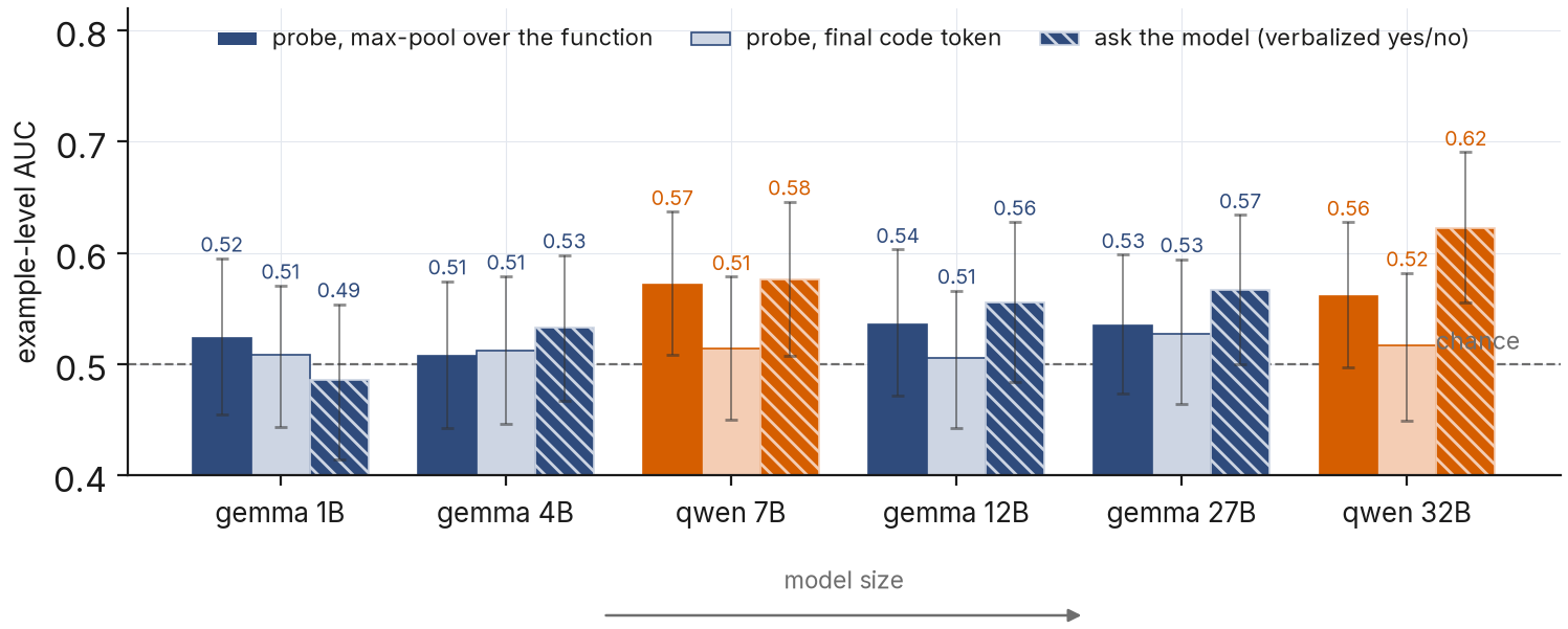
    • In particular, using simple max-over-tokens or final-token-probe performs near chance for example-level evaluations.
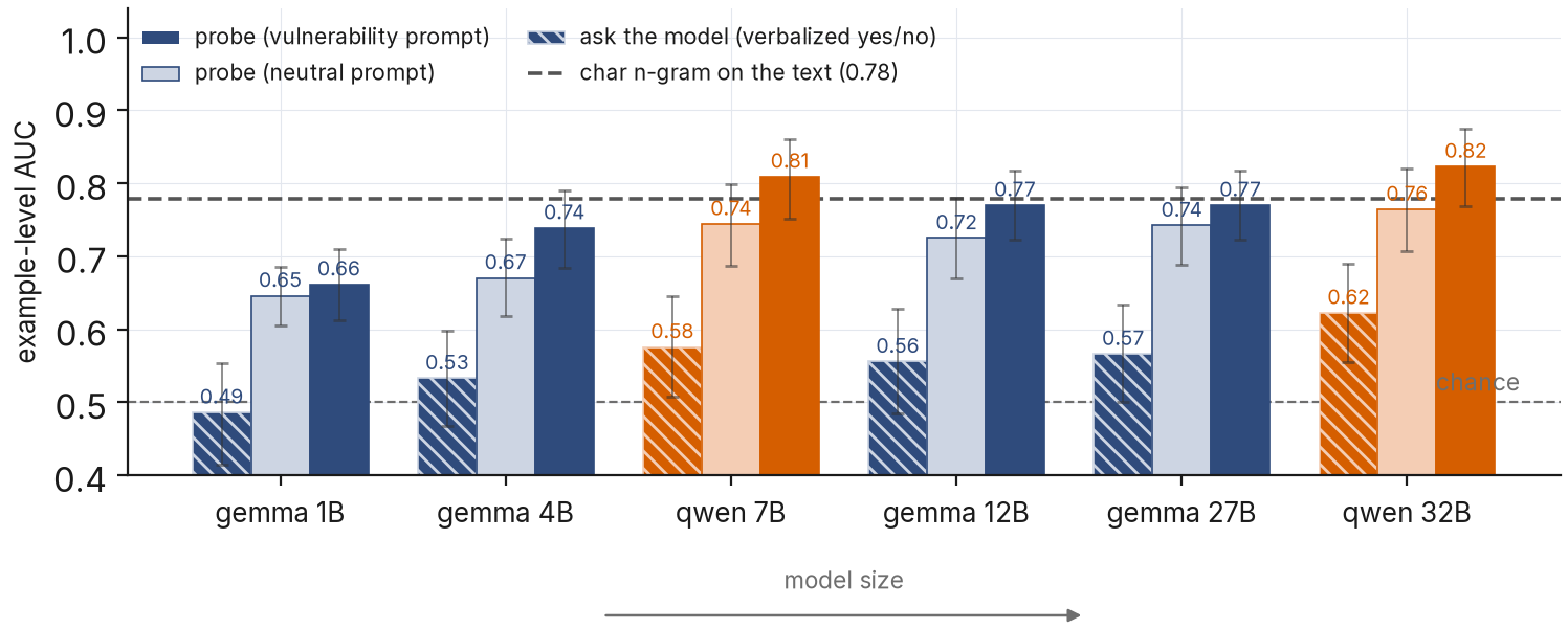
    • Example-level performance is recovered when using specific prompts and probing start of assistant message, but requires specific prompt for the best performance.
  • I tried different probing methods like MLP probes, verbalization, and k-ensembles of linear probes. MLP probes had slightly higher AUC, but come with reduced interpretability and higher training cost.
  • I controlled for biases in the dataset, and simple baselines. I found out that the vulnerability probe on a fixed dataset is likely the wrong evaluation.
    • Looking at individual predictions, the probe matched code patterns more closely than model understanding of vulnerability.
    • A baseline trained on raw text scores higher on token AUC.
    • A language-based baseline got 2/3 of the probe’s performance in AUC (dataset imbalance) in the general evaluation. This led to within-language evaluations.
• Future work
  • Followups on this dataset: look at better metrics like accuracy@1%-FPR, pair accuracy to see how bad the probe would be in reality.
  • Next candidate proxy task is evaluating probes on model-generated code directly, which is closer to agentic workflows.
• Conclusion
  • Linear probing should not be used to detect vulnerabilities in individual pieces of code. Lexical baselines are likely to perform better and cost less.
  • This project did not determine whether LLMs encode in activations that they are writing vulnerable code.
  • My takeaway: it’s important to aggressively control on dataset biases and try simple baselines.

Note: This project was performed as part of Bluedot Impact’s Technical AI Safety Project course.

Dataset

I started with SVEN (He and Vechev 2023), a dataset of vulnerable/patched function pairs by He and Vechev, with each pair’s vulnerability type (CWE) marked. I turned it into a token-level dataset by marking the tokens removed in the safe code as positive in the vulnerable function. Mechanically: SVEN records which characters the fix changed, and I intersect those character ranges with live-code regions and map them onto each model’s tokens through the tokenizer’s offset mapping, so every model is trained and scored against the same label axis.

He, Jingxuan, and Martin Vechev. 2023. “Large Language Models for Code: Security Hardening and Adversarial Testing.” Proceedings of the 2023 ACM SIGSAC Conference on Computer and Communications Security (CCS). https://arxiv.org/abs/2302.05319.

SVEN has 715 pairs (1,430 functions) over 9 CWEs (vulnerability types); by language it is composed of 756 Python, 574 C, and 100 C++ functions. The two biggest CWEs are SQL injection (CWE-089, 203 pairs, all Python) and command injection (CWE-078, 105); the memory-safety side is out-of-bounds read (CWE-125, 103), NULL dereference (CWE-476, 65), use-after-free (CWE-416, 56), and out-of-bounds write (CWE-787, 47). Note that CWE/language are correlated, this became important when evaluating with language baselines.

For more in-depth understanding, I split the data by CWE (vulnerability type) and by language, and isolated the subtractive pairs (pairs where the fix changes existing code instead of only adding a check); 478 of the 715 pairs are subtractive, and the other 237, a third of the dataset, only add a guard. Note that in subtractive pairs, there is no positive token, just a positive example as a whole and negative tokens.

To cross-check my results, I used the similarly structured PrimeVul dataset (Ding et al. 2025), which provides C/C++-only vulnerable/patched pairs I could process the exact same way. PrimeVul is bigger and broader: 4,704 pairs across 111 CWEs, with a similar subtractive fraction (54%), giving it about five times SVEN’s volume of pairs with markable vulnerable tokens.

Ding, Yangruibo et al. 2025. “Vulnerability Detection with Code Language Models: How Far Are We?” Proceedings of the 47th International Conference on Software Engineering (ICSE). https://arxiv.org/abs/2403.18624.

Probes and the metric

I trained linear token probes on the residual stream across layers. Setup was supervised training with custom loss taken from the hallucination probes paper (Obeso et al. 2025). The loss starts off as BCE on tokens (detect vulnerable tokens individually), then anneals to a BCE on span-max over positive tokens (detect at least one vulnerable token in a given example). I swept layers per model and picked the best layer on validation AUC. Splits are performed at the pair level to avoid data leakage.

Obeso, Oscar, Andy Arditi, Javier Ferrando, Joshua Freeman, Cameron Holmes, and Neel Nanda. 2025. “Real-Time Detection of Hallucinated Entities in Long-Form Generation.” arXiv Preprint arXiv:2509.03531. https://arxiv.org/abs/2509.03531.

I used a linear layer probe (a single weight vector per model) trained on cached activations with AdamW at learning rate 1e-3 for 30 epochs, with the loss blend moving linearly from the per-token term to the span-max term over training. The layer sweep covers every layer of every model (26 to 64 layers depending on size), and the validation-based selection is close to the best-on-test layer for every model (appendix).

For evaluation, I used ROC-AUC over individual tokens, computed only on live code (comments and trivial tokens are filtered out and excluded from scoring) as the evaluation metric. 0.5 represents chance; 1.0 would rank every vulnerable token above every clean one. Note that ROC-AUC also means the probability that a positive example is ranked over a negative example. Concretely, the live-code filter uses tree-sitter to drop comments, import/include lines, function signatures, decorators, and preprocessor directives, about 30% of all tokens. All test numbers below come from a held-out pool of 292 functions (146 vulnerable, 146 patched): roughly 76,000 live-code tokens, 4,160 of them positive.

Initial results

Token-level probes get 0.75 to 0.82 token AUC across model sizes and families. Interpretation of AUROC tells us that it’s 80% likely to separate positive examples from negative examples.

Figure 1: AUC per model: linear probe (bars), MLP head (diamonds).

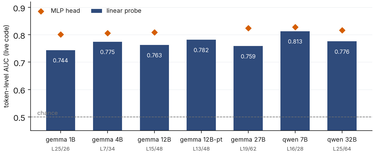
Interestingly, the 7B Qwen model beats its 32B counterpart, and the validation-selected best probing layers are mostly early-mid (roughly 20 to 40% of depth) rather than mid-late as would be expected from semantic understanding.

A caveat: This total AUC score misses per CWE/language differences. For example, SQL injection scores 0.92 while use-after-free sits at 0.52. When split by language, Python is at 0.81 AUC while C is at 0.59 AUC.

Grouping the CWEs into two families makes the split clearer: every probe detects injection-class bugs well (0.85 to 0.91) but performs near randomly on memory-safety bugs.

Figure 2: Per model, the probe’s token-level AUC on injection-class CWEs (SQL, command, path, XSS; green) versus memory-safety CWEs (out-of-bounds read, use-after-free, NULL dereference; orange). The blue tick denotes the score from the previous figure. Each family bar is the CWE-pooled AUC scores. Note that negatives include other CWEs.

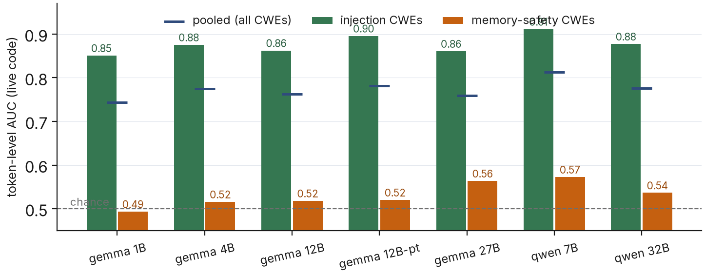
An imbalance of performance between these two are expected due to SVEN’s imbalance of vulnerability types. The ratio of injection to memory tokens are 2.2:1. However, this does not explain the near-chance performance in memory type vulnerabilities. I believe the rest of the loss of performance is explained by the difficulty of detecting memory vulnerabilities, as well as the confounder that memory vulnerabilities may be an artifact of the codebase architecture, and not a single function.

Above comparisons were done with token-level predictions (does this token cause vulnerabilities?). However, trying to generalize this to example-level predictions (is this function vulnerable?) fails with naive approaches. Using a simple final-token probe or probe maximum logits over an example is random chance compared to token-level AUC’s 0.70-0.80 figures.

Figure 3: Per model, example-level AUCs for max-pooled predictions over all tokens in a function, final-token probes. Green dashed line shows the token-level AUC figure (inherently different task, shown to contrast the difference.)

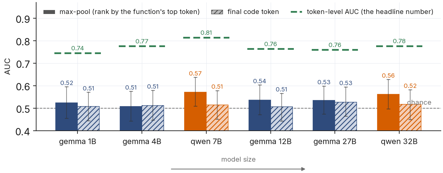
Later in Figure 7, we see that verbalization performs better than this naive approach and that probe performance can be improved with extra prompts.

Overall, this is a slightly positive result with injection/Python vulnerabilities being a potential candidate to use probes for (in token-level contexts). To better understand probe performance in this project, I decided to dive deeper into the nuance behind this result. Next, I attempt to break this down: first the probe side (can different probe architectures do better?), then the evaluation side (what are the biases in the dataset? do training individually on vulnerability types perform better? what are we detecting? do the findings replicate cross-dataset?).

Could a stronger probe perform better?

First, I tried to answer the question: Can we get better detection by using bigger probes or bigger models?

Variations on model did not meaningfully change the AUC results:

• Instruction tuning: a probe on the base 12B model matches the instruct version (0.782 vs 0.763).
• Scale: 1B to 32B spans 0.744 to 0.813 with no trend (Figure 1).

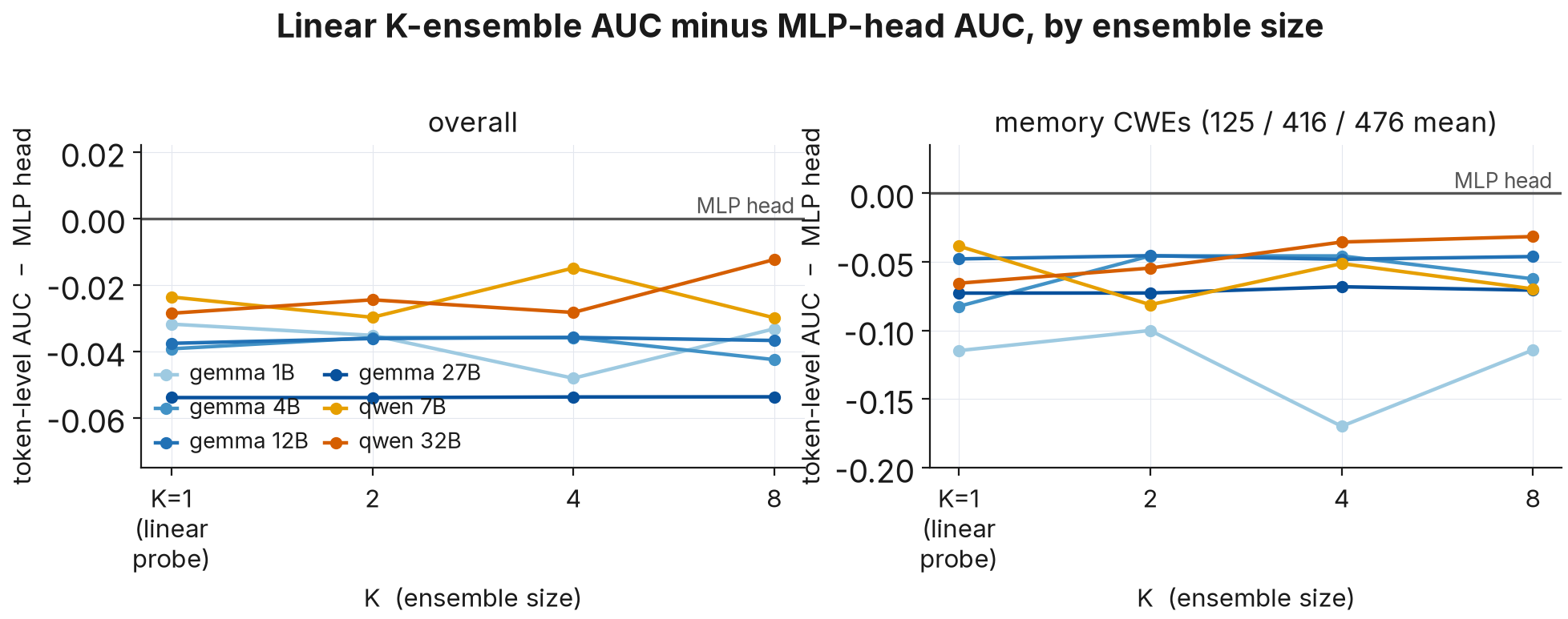
Then, I experimented with probe architecture starting with MLPs. The MLP probe is a two-layer head (hidden width 256 or 512, 1 to 3M parameters depending on model). I swept across layers, and got 0.79 to 0.83 AUC on every model. MLPs have a lead over linear probes on all variants. However, their failure mode is also similar, catching injection family bugs, but missing memory vulnerabilities.

Figure 4: Linear probe vs MLP probe

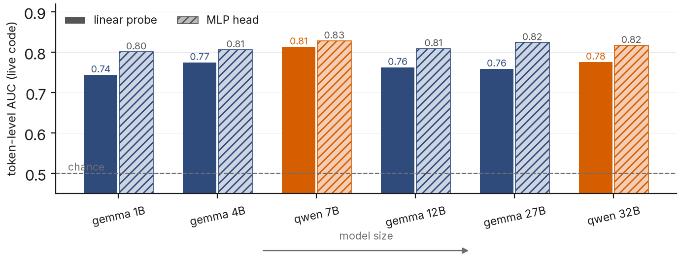
To see if this performance could be recovered by a more interpretable alternative, I tried K-ensembles of linear probes. This setup replaces the single linear direction with K directions (1, 2, 4, 8) directions trained jointly. The per-token scores from each direction are combined by either max, logsumexp, or a learned gate (best chosen for eval).

To better regularize joint training, I forced the K directions apart with an orthogonality penalty. The penalty worked with mean cosine similarity falling to 0.002 but the AUC did not change.

Overall, the results are unimpressive. The only notable improvement was Qwen-32B where the best ensemble (K=8, logsumexp) gained +0.016 but fell short of the MLP. For an interpretable probe, it seems combining multiple linear probes do not help.

Figure 5: Linear K-ensemble AUC minus the MLP head AUC showing how much ensembles recover MLP performance. The zero line is the MLP head. On both overall and memory CWEs, linear probes are below MLP. On Qwen2.5-Coder-32B, linear probes approach MLP with increasing K. (Absolute score ranges: overall ensembles 0.75–0.81 vs MLP 0.80–0.83; memory ensembles 0.44–0.58 vs MLP 0.57–0.63.)

Next, I decided to investigate per-example performance more closely. First, I tried verbalization. With this method, the model is asked if the code is vulnerable, and P(yes) is read in a single forward pass. Verbalization performed better than naive max-over-tokens and final-token approaches for increasing model sizes, however the example-level performance was still disappointing.

Figure 6: Verbalization compared with naive example-level application of the token probes. Results are near-random for all but the Qwen 32B model.

Next, I tried a combination approach: probing on the final assistant turn token with specific prompts. I compared two simple prompts: 1. asking the model neutrally (What do you think about this code?) 2. asking the model about vulnerabilities (Is this code vulnerable?), then probing on the assistant turn’s starting token. These approaches outperformed verbalization by a surprising amount. Qwen 32B’s performance exceeded even that of the baseline (char-n-gram).

Figure 7: Per model, example-level AUC comparing probes on neutral and vulnerability-related prompts against asking the model. Upper dashed line (0.78) shows what a lexical-only baseline achieves.

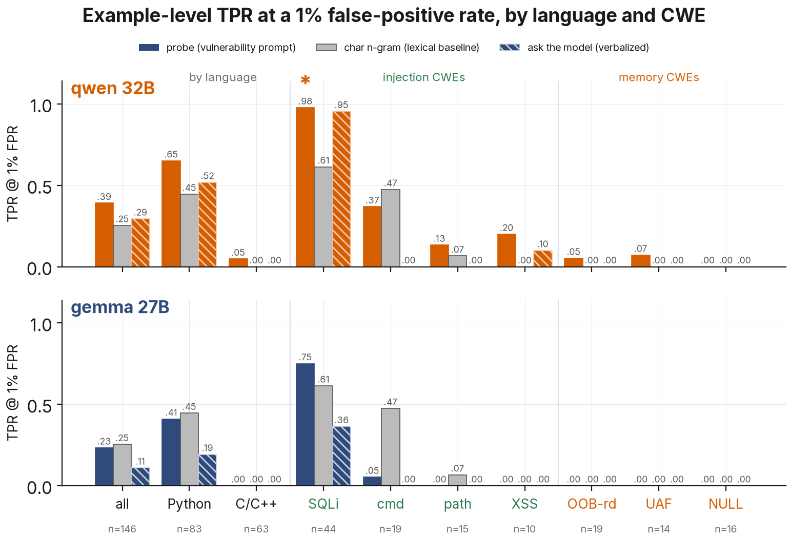
AUC is not the best metric for understanding the performance of production-candidate probes. Other metrics like TPR@FPR=0.01 are often used in cases where false positives are undesired and are costly. A good probe should have high TPR at low FPR so that the people monitoring are not overwhelmed by false positives while missing critical positives.

Looking at the promising candidates from AUC, the TPR@FPR=0.01 is disappointing across CWEs, with particularly bad performance at memory and C/C++ splits. The only production-usable probe seems to be for SQL injection with Qwen 32B. On Qwen 32B, the probe is evidently outperforming lexical baselines in all but the command injection vulnerability whereas the Gemma probe is not as promising. In general, I saw that Qwen probes outperformed Gemma across sizes, which could be explained by Qwen’s focus on coding during training.

Figure 8: Example-level TPR at a 1% FPR threshold, by language (left) and CWE (right). Filled accent color denotes the best probe, gray bar denotes the fixed lexical baseline, dashed fill denotes the verbalized baseline.

Investigating the probe’s classifications

I decided to fix a threshold to see what the probe finds and does not find systematically across models. Threshold was fixed to be the F1-maximizing one on training tokens. For an example-level evaluation, I gave the probes an unfair advantage: I maxed the score over oracle vulnerability-relevant tokens, and used that max score to classify. For token spans, I considered false-positive spans where the probe fired but the range was not in the diff range.

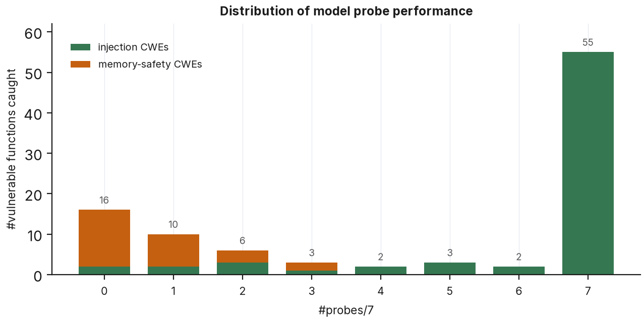
Looking at the 97 held-out vulnerable functions, for all seven models’ probes, the performance turns out to be similar among probes: 55 of the 97 functions are caught by every probe and 16 by none. The always-caught set is purely injection (43 of them SQL injection); the never-caught set is mostly memory-safety. The probe performance is clearly biased towards injection, with very little memory vulnerabilities being detected. Looking at the false positives, 3,125 of the FP spans land on patched code, and the cross-model ones are 96% injection pairs.

Figure 9: Probe classification performance across the 7 model-probes (from initial results), colored by vulnerability type.

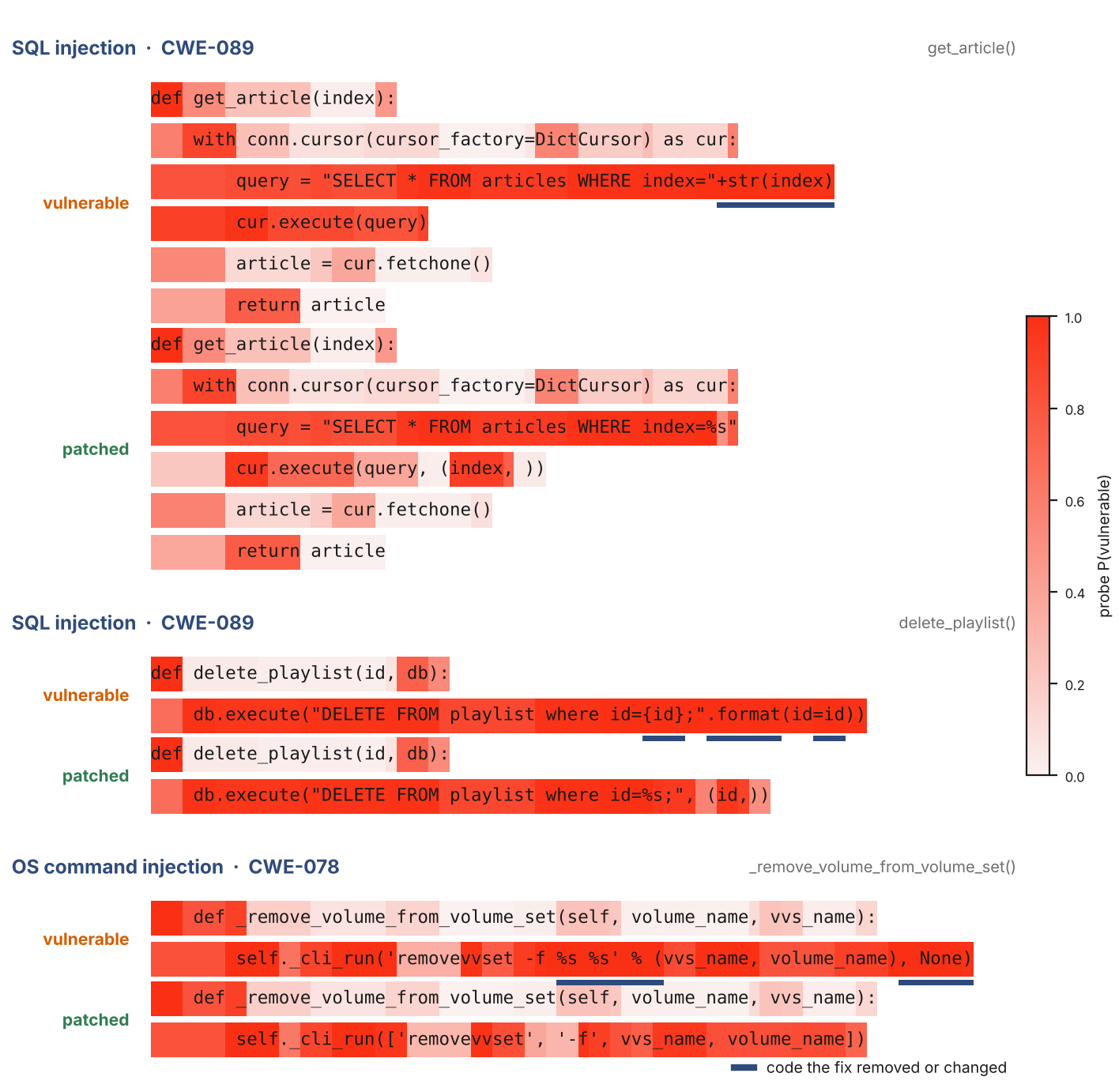
The probe seems to be matching string patterns more than an understanding of vulnerability. It’s easier to see this with matched pairs. Figure 10 shows examples of 2 SQL-injection and 1 OS-command injection vulnerabilities. The probe is unable to capture the semantic fix. It keeps detecting SQL or command string at peak scores.

Figure 10: Three held-out functions, each above its own security fix (Qwen2.5-Coder 32B). The probe (red) paints the whole SQL or command sink string in both versions; the underline marks the true positive tokens. The probe fires on the entire string, not on the edit that removes the vulnerability, and barely shifts between the vulnerable and patched versions.

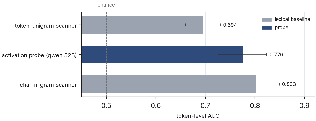
Since string matching seems to be the dominant mode of detection, I selected lexical baselines that when exceeded, would indicate that model understanding could be involved. I started with text-only scanners on the same splits: 1. a token-unigram logistic regression (token identity alone), and 2. a character 3-to-5-gram logistic regression reading a ±48-character window around each token. Note that the scanners are deliberately favored, because I wanted a solid lexical baseline: char-n-gram’s input window sees to the future whereas model activations are causal in sequence, and baselines train on fine-grained per-token labels whereas the probe’s loss anneals to the coarser span-max loss (one label per span).

As a result, the char-n-gram baseline beats the probe, 0.803 [0.748, 0.849] vs 0.776 [0.725, 0.824], and even the single token baseline reaches 0.694. This result tentatively shows that the probe does not beat using simple lexical patterns. Although it has to be said that the input code is out of distribution for the model, as the code has not been generated by the model, thus there may not be any understanding of vulnerability to be detected.

Figure 11: Text-only scanners vs the probe.

Language imbalance

Another problem with looking at the total token AUC is that the SVEN dataset is langauge-imbalanced. In SVEN, 378 of the 410 injection-vulnerable functions (92%) are Python and SQL injection is Python-only, while all 305 memory-vulnerable functions are C/C++. The net effect is that positive tokens are about 4× denser in Python.

An important baseline this suggests is to use language as the score: score every token 1 if its file is Python, 0 otherwise. In token-level AUC, this scores 0.677 AUC. In margin-over-chance terms, (0.677 − 0.5) / (0.776 − 0.5), is about 64% of what the probe achieves, with zero vulnerability information.

Figure 12: The language baseline vs the best probe (Qwen2.5-Coder 32B).

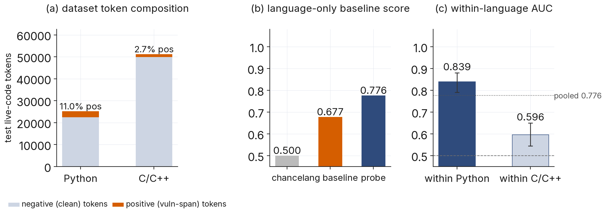
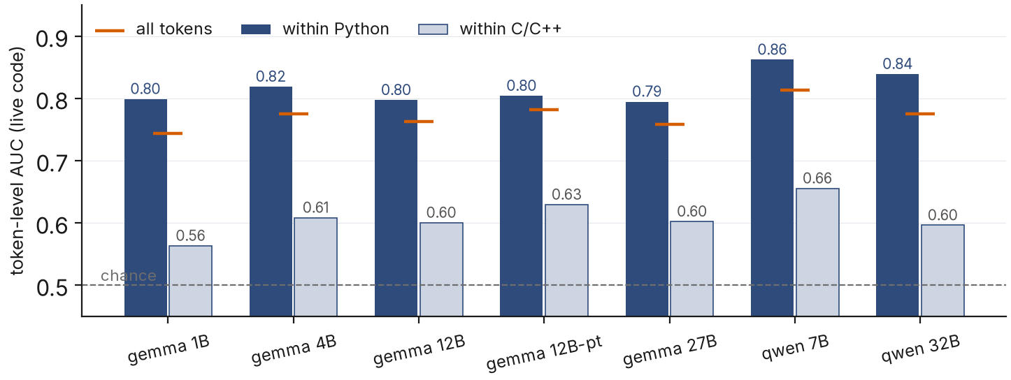
Thus, I break down the dataset by language to see the language-invariant token AUCs. Probe performance is strongly biased towards Python: 0.80 to 0.86 within Python, 0.56 to 0.66 within C/C++, on every model.

Figure 13: Within-language AUC, all models. Orange marks: the pooled (original) score.

Pairs without positive tokens

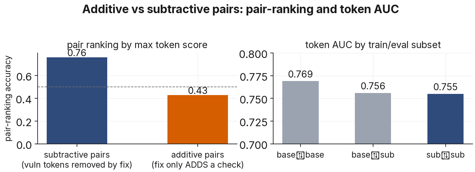
A third of SVEN diffs add a check (a bounds test, a null guard), rather than remove vulnerability-causing code. The before-version has no vulnerable token to mark, thus positive labels don’t exist for these pairs. To investigate the effects of this subset, I separated the dataset into so-called “subtractive” and “additive” subsets. The subtractive pairs have some code that’s removed in their safe version whereas additive pairs don’t.

Now, I look at the example-level pair ranking accuracy: rank the vulnerable function above its own fix by its max token score. The accuracy comes out worse than random for additive pairs as can be expected (there are more tokens that increase probability of hitting a larger logit). The control is restricting to subtractive pairs, and it costs nothing: 0.756 vs 0.755, with the gap far inside cross-validation noise (appendix). This is an honest blind spot of the whole token-probe approach: missing-check vulnerabilities are invisible to it.

Figure 14: Additive pairs: ranking at chance (left); dropping them costs nothing (right).

Cross-validation on PrimeVul (WIP)

This section is a work-in-progress, will be completed today.

Next steps

The most important design gap in this study is that probes were trained on single functions out of repo context; this study never checked whether the model holds any belief about them at all. Some examples are impossible to reason with vulnerabilities as well (memory vulnerabilities depend on function usage). The negative results have more than one reading: the probe catches lexical patterns, model has no vulnerability understanding to read, or the vulnerability understanding happens at different tokens.

Some next experiments that could be performed that I did not pursue, to better understand the results.:

• Random-direction probe distribution: the AUC distribution of random unit vectors per layer, with the trained probe reported as a percentile of that null (the sleeper-agents paper checked this; random directions hit 0.95 there). This would demonstrate how unique the direction that the trained probe catches.

• Pivoting to generation-based probing: probing generation-time states on model-written code with labels from analyzing the code directly. The monitor the North Star calls for should probe in-distribution code.

Conclusion

Activation probes for code vulnerability, as evaluated here, mostly seem to rediscover textual patterns and are unreliable for detection of vulnerabilities as demonstrated in the SVEN dataset. There is still a lot of pending work to narrow down whether LLMs know when they’re writing vulnerable code, but it’s clear that LLMs should not be used to detect vulnerabilities in existing isolated pieces of code. The learnings of this project are mostly in understanding dataset quirks and experiment controls that should be included in probe research. Baselines like text-only scanners, composition nulls, and experimentation with multiple metrics, controlling for covariates in the dataset as well as cross-checking on a secondary dataset are key steps in probe research.

Supplementary

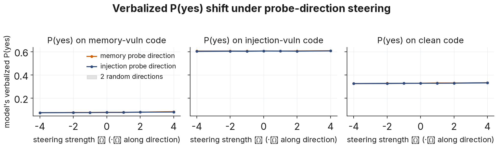
Steering is a no-op: adding ±4σ along the probe direction at the probe’s layer moves the model’s verbalized P(yes) by at most +0.011 on all four models tested, indistinguishable from random directions; pushing to ±64σ destabilizes generation generically (clean code’s P(yes) rises more than vulnerable code’s). The direction is a correlate, not a control knob.

Figure 15: Steering at ±4σ: verbalized judgment unchanged.

Appendix: validation details

Checks that don’t change the story but back it up:

• Masking no-op. Excluding comments and trivial tokens from training (not just from scoring) changes test AUC by between −0.013 and +0.002 across all 8 models, and the code-only score is not below the all-token score on any model. The live-code restriction is honest scoring, not probe rescue.
• Layer selection. Every layer of every model was swept (26 to 64 probes per model). Selecting by validation token-level AUC lands within 0.025 of the best-on-test layer on all 8 models; selecting by example-level AUC, the earlier protocol, picked near-random layers (up to 0.065 below the best).
• Loss annealing strength. In the span-max loss, annealing weight α was sweeped. α=1 beats α=10 by +0.012 to +0.033 example-level AUC on both models tested; token-level AUC is flat in α.
• Subtractive-restriction stability. The 0.756-vs-0.755 comparison was re-run as a 5-fold × 3-seed cross-validation (15 retrainings): fold-to-fold standard deviation is about 0.024 (Qwen) to 0.04 (gemma), and every base-vs-subtractive training gap is far inside it.
• Saved-logit rescoring and reproduction gates. Every deconfound (language, matched-patch, scanner comparisons, PrimeVul) re-scores per-token logits that were saved at extraction time, on CPU, with no retraining. Each one first had to reproduce the historical headline numbers from those saved logits (to within 0.0003 for the language rescore; exactly, bit for bit, for the matched-patch and PrimeVul re-runs, 48 of 48 cells) before any new slice was reported.
• One bookkeeping note. Qwen-32B layer 25 has two legitimate probe fits in the project: 0.776 (the canonical headline) and 0.788 (a refit that serves as the ensemble and MLP experiments’ own baseline). The deltas in the probe-architecture section are against the 0.788 baseline; everything else in this post uses 0.776.